Building Dashboards in Excel > Part 1 - Valid data

When you create dashboards with Excel, valid data is the key to succes! This article is about Excel and data, what you have to know about valid data and what options Excel offer to be sure that you will work with valid data.

Excel is a great tool when you have to analyze large amounts of data. Whether this is financial, product or customer information does not matter. Excel will handle it all. In most situations, the data to be analyzed is presented in a table. Or a database?

Excel users very often speak of a table or a database assuming that they are the same thing. This is incorrect; they are quite different! So what about the terminology being used. Do we speak of a table, or do we speak of a database?

According to Wikipedia, a table is an ordered arrangement of rows and columns, where a database is an organized collection of data. To be more exact: Multiple well-organized tables, which are connected by some kind of record key, make a database.

Excel at the other hand, is about ranges and tables, does not mention the word database, but does discuss a data model. This might make it a bit more complicated, so here is what you have to know. An Excel range is the ordered arrangement of rows and columns, where an Excel table is a range with special features.

Being able to implement Excel’s powerful table features makes working with data in Excel even more interesting, but these features will be covered extensively in an article about Excel and Tables. Because a range and a table are so often seen as the same thing, I will, for the sake of simplicity, in this article refer to a table.

Excel handles data, or records stored in a table very well, but only when you keep the following limitations in mind:

• The number of rows, or records, can’t be more than 1048576
• The number of columns, or fields for a record, can’t be more than 16348

When you have to work with a set of data that exceeds these limits, the standard version of Excel is not suitable to the task. You may solve these issues with the PowerPivot utility that Excel offers, but other than that, you are stuck with using a different tool. In some cases, Microsoft Access might be a good candidate.

This does not mean that a table with a million records and 250 fields is a nice alternative to work with. Internal PC memory and processing power might then become a bottleneck. As a rule of thumb, you should consider a table with 500000 records, containing 32 fields, a decent number to work with.

Building a table involves more than entering data. A proper design is crucial to its success. Especially when you have to work with a large set of data, it is wise to keep the following rules in mind:

• Use a clear description for each field on the header row (the first row)
• Use only one row as the header row
• Don’t create empty rows (records) and columns (fields), for it splits the table
• Design columns in such a way that each individual entry has the same format
• Freeze the header row so that the field labels are always visible
• Sort the table data in a logical order

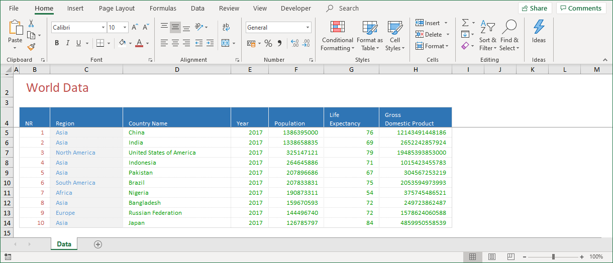
When you follow these principles, you can design a well-structured table with data. Figure 1‑1 shows such a table.

So in Excel, it’s all about data. Lots of data is one thing, big data is another thing, but valid data is the main thing. This sounds simple, but when you are analyzing data, valid data is the key to success! Invalid data is where many of the problems begin.

It is the main reason for failure.

Sometimes, when you start a project, your first effort is to collect data. That may not always be so easy. In many occasions, people from multiple departments within the same company, are entering data into different data systems.

When it is your task to analyze data, you may have to merge data from different data systems into one big table. This might seem disappointing, but it is something that you will have to manage too. At least, that is my experience!

I have done projects for many companies in all kinds of fields. No matter what I had to do, I never had the luck of working with just a single source of data to be the single source of truth. I always had to piece my data together.

It might be a bit exaggerated to say that you can’t trust your data, but I have been in many situations where data that was imported into Excel, was simply not checked. In some cases, the financial errors and miscalculations because of this added up to millions of euros. This is something that no one would like to have to deal with and so it is clear that you should always verify your data before you start doing anything in Excel!

So, where might invalid data come from, or how can it occur?

Invalid data might come from text files where data is imported as text. This includes text, as well as numbers. The imported numbers, the so-called “text-numbers” can’t be summed, or analyzed, because it is text.

Entries may also contain obsolete spaces. These are spaces that are entered before or after a value, making the entry invalid. Fortunately, as you will see further on, Excel offers a couple of tools to correct these issues. These tools will ensure that you can work with valid data. Data that is formatted as it should be and that is ready to be analyzed. Most of these tools are pretty simple but also hardly used. So, what do we have available?

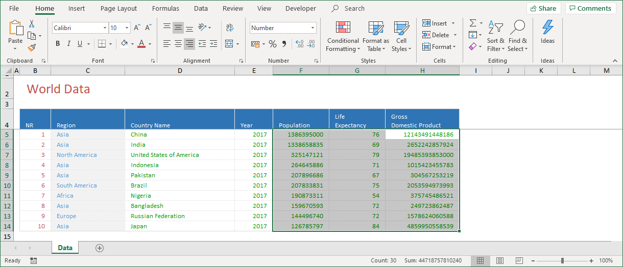
The first part in working with valid data is to check whether that data is indeed valid or needs to be corrected. Consider the following table with data.

You have learned from the previous chapter that this data is useless, as all the numbers are formatted as text and can’t be summed. The main indication for this, is the little green triangle at the top left corner of a cell.

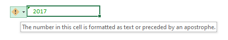
When you select a cell with such a green indicator, an information sign appears. When you hoover your mouse over this information sign, you get to see the information about what might cause the error. In this case it is the fact that: “The number in this cell is formatted as text or preceded by an apostrophe”.

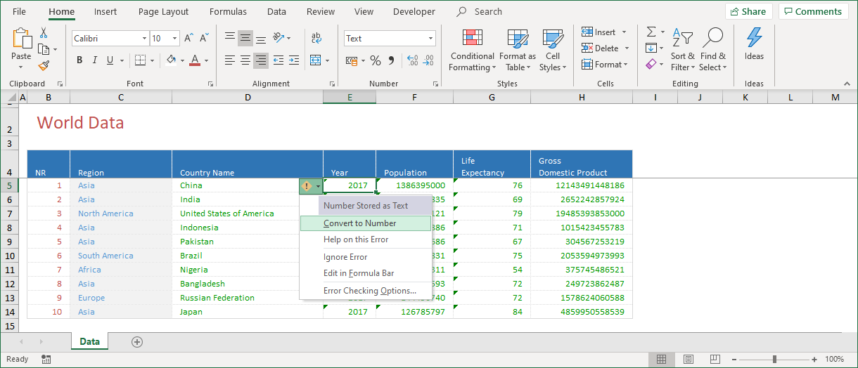
Next to the information sign, a down arrow appears as well. When you click the information sign, a menu unfolds showing options that you can choose to solve the issue.

The first option “Number Stored as Text” indicates the real issue. This option is greyed out, as you can’t click or select this the option.

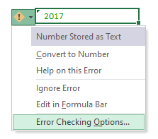
The last option, Error Checking Options… is the most interesting option. It might reveal why some errors are unnoticed and why people proceed with their work even though their data is invalid!

When you click the option Error Checking Options…, the Formulas section from the Excel Options dialog appears.

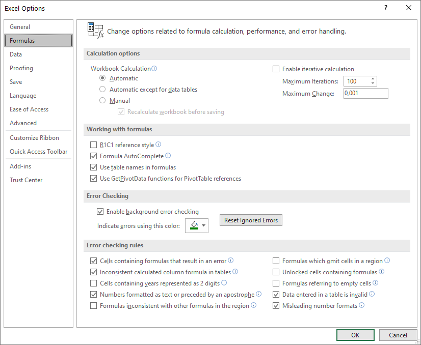
The Error checking rules section is the most important section. It offers ten rules, or options that indicate how Excel handles possible error issues. All these rules are optional and it is you, the user, that decides whether they are active or not.

The rules that you have chosen to be active, are the rules with a checkmark. Figure 2‑4 shows four active rules. The “Numbers formatted as text or preceded by an apostrophe” is one of them. The result of this is the fact that cells containing a number formatted as text, are now indicated with the little green triangle in the top left corner of the corresponding cell. This rule is, in my view, a must have feature to select, as it clearly indicates numbers that you can’t use in calculations!

The opposite, regrettably, can also occur. An inexperienced user may, without knowing why, choose to not check this feature, leaving the worksheet with fewer indications about invalid entries! This is where the misery might begin.

Let’s say that this is the case. What can you do to avoid working with invalid data?

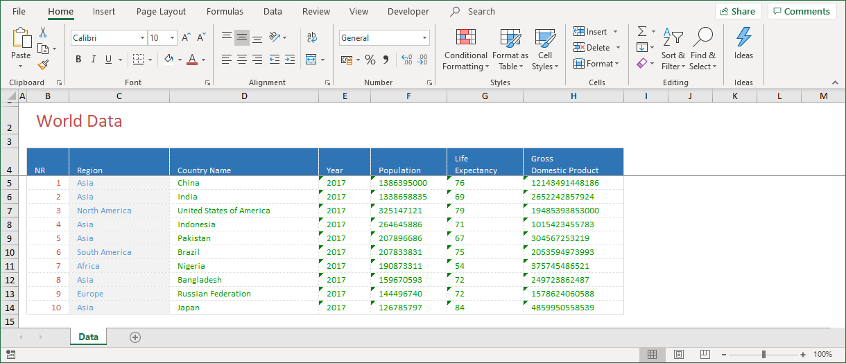
When the option “Numbers formatted as text or preceded by an apostrophe” is unchecked and Excel does not show a little green triangle in the top left corner of a cell that contains a number formatted as text, the worksheet might look like the one in Figure 2‑5.

Figure 2‑5 shows a worksheet where a lot of numbers are formatted as text and right aligned. But which? How do you know whether this data is valid? How do you know that the numbers that you see, are valid numbers formatted as a number?

The thing is that you don’t. You could have been the lucky one that received a table with valid data, but you could also have been less fortunate and received a table where a lot of numbers were formatted as text and right aligned!

Now whether you are the lucky user or not doesn’t matter. All users, in my view, should follow a couple of checks before they proceed working with the data displayed in Figure 2‑5. These checks are pretty simple!

When you quickly want to see if all of your data is formatted as a number, you should select the cells that you want to check and take a peek at the status bar.

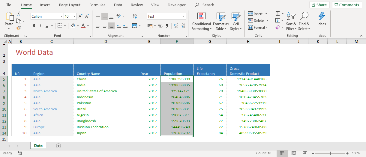
In Figure 2‑6, I selected all the values for the Population field. The status bar indicates that I selected 10 items, as it shows a Count of 10. The fact that the status bar only shows a Count, indicates that the format of this values is text. If the format of this values would have been a number, the status bar would also show a Sum!

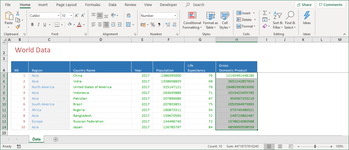
In Figure 2‑7 I selected the values from the Gross Domestic Product field. The status bar clearly indicates that these values are indeed formatted as a number!

Some people use the ribbon as a reference to the number format. Although this is just another way of getting the same information, you should be careful, as the Number Format section from the ribbon might fool you! Consider the example shown in Figure 2‑8.

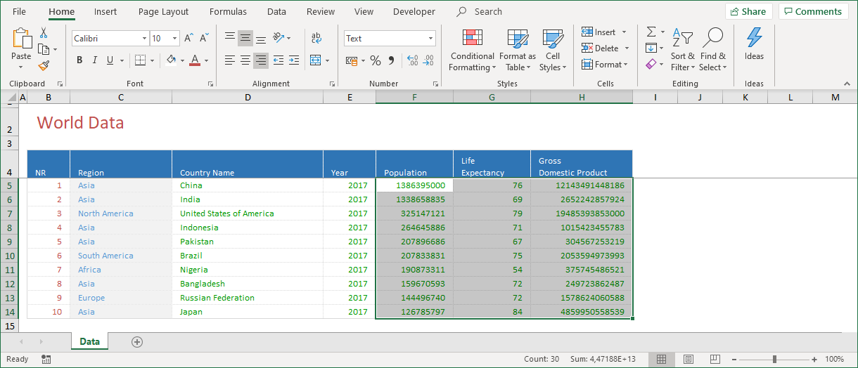
You know from the previous pages that the values from the Population field are formatted as text, but that the values from the Gross Domestic Product field are formatted as a number. Why then, does the ribbon inform you that the selected cells are formatted as Text?

The answer to this question is about the active cell. This is the cell from which you started the selection. In this case the top left cell from the selection, which is indeed formatted as Text.

In case you had started with the Gross Domestic Product field and extended the selection to the left, the ribbon would have shown a different number format. Then the ribbon would have informed you that all of the values were formatted as a number, which is not true!

So the status bar and Number Format section from the ribbon don’t seem to be appropriate features for a correct indication about the real number format. What then could you use to find out what the number format of a range of cells really is?

The best way to check the number format of a range of cells, is to use a combination of the control and arrow keys. This is how that works.

Assume that you want to check the number format of the values in the Population field shown in Figure 2‑9. To do so:

• Select the first value of the Population field
• Press the CTRL and SHIFT keys, but don’t release them
• Press the down arrow key, to select all continuous cells (to the end, or bottom)
• Release the CTRL and SHIFT keys
• Press CTRL 1, to display the format cells dialog

If all went well, the following dialog appears:

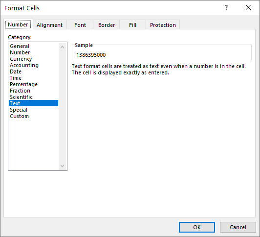
The Number tab from the Format Cells dialog shows a preview of the number format of the selected cells. From the Category list of the Number tab, the Text option is selected. It is also colored blue. Next to that, the exact value from the first selected cell (the active cell) is shown as a Sample.

This seems to be correct, but how do you know that the Format Cells dialog indeed displays the right number format?

This can be checked with a simple test. Instead of selecting the values from one field, you can select the values from multiple fields. Just as what you did in the examples in Figure 2‑8 and Figure 2‑9, you can start with the first value of the Population field and extend the selection to the right and all the way down. This works as follows:

• Select the first value of the Population field
• Press the CTRL and SHIFT keys, but don’t release them
• Press the right arrow key, to select all continuous cells (to the right)
• Press the down arrow key, to select all continuous cells (to the end, or bottom)
• Release the CTRL and SHIFT keys
• Press CTRL 1, to display the format cells dialog

Now this is what the Format Cells dialog looks like after you selected this range of cells.

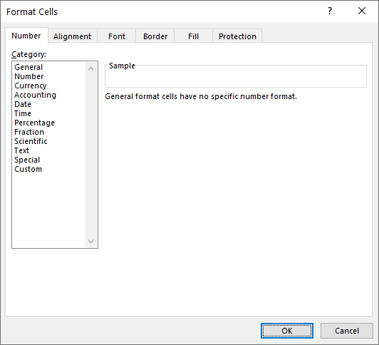
There is no number format selected at the Category section of the Number tab, nor does the dialog show a sample value. The fact that these features don’t show anything at all, indicate that the selected cells have different number formats!

With this in mind, you can create a set of rules to check the number format of cells.

• Identify the fields, or columns with data, that you want to check
• Check only one field at the time
• Select the first, or top cell from the field that you want to check
• Use a combination of the CTRL, SHIFT and down arrow keys to select the whole range of cells

Use the Format Cells dialog, by pressing CTRL 1, to check the number format of the selected cells

By following a set of rules to check the number format, you found out that a lot of fields in the table contained numbers that are formatted as text. How do you convert these so called text numbers?

There are a couple of ways to convert text numbers to normal numbers. When you need to convert just a few text numbers, the easiest way is to click the drop-down arrow next to the exclamation sign and select Convert to Number.

Converting text numbers by selecting individual cells is a time-consuming operation, so there must be a faster way to solve that issue. Indeed, there is. You can also select all cells that need to be converted, click the drop-down arrow next to the exclamation sign and select Convert to Number.

However, the Convert to Number operation won’t work when the top left cell of the selection (the active cell) does not contain an error value, like a text number. In that case, the error checking option menu won’t appear!

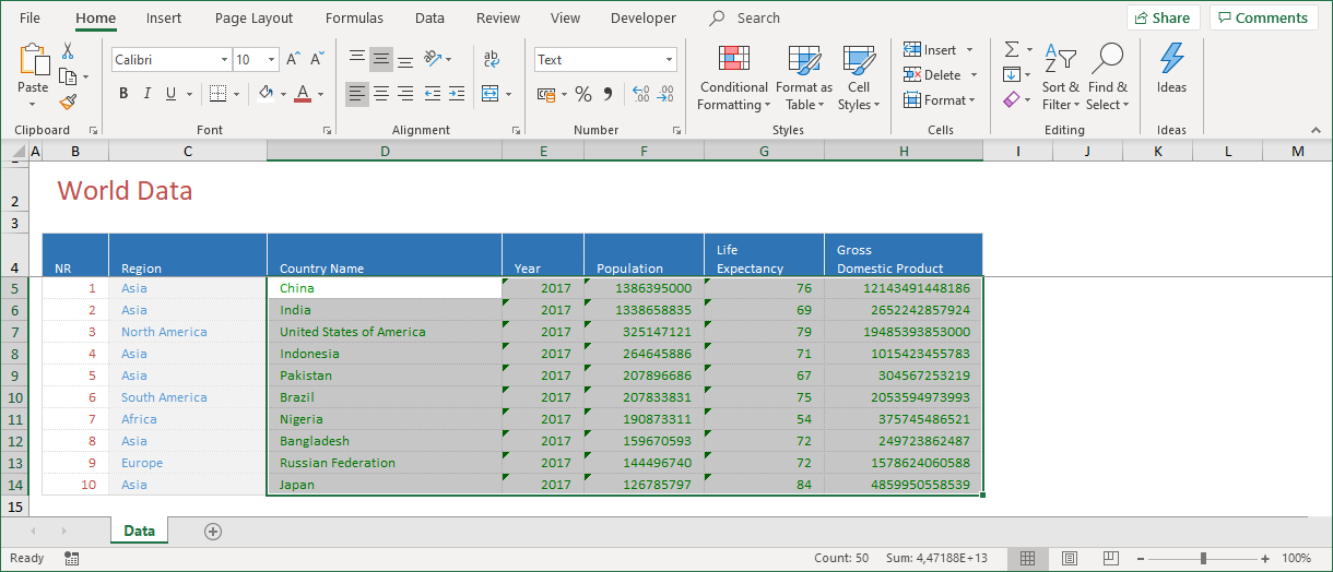
Figure 3‑2 shows an example of a selected range of cells with numbers formatted as text. In this example, the cell containing the Country Name China is correct, so there is no need to give a hint to a possible error value. This error would also occur when that cell is empty.

Because of this, the little green triangle at the top left corner of the cell is not visible and the error checking menu can’t be activated directly from that cell.

When you have to convert a lot of text numbers, there are a couple of smart ways to do so. One of them is to use the Paste Special functionality!

When you perform a standard copy and paste operation, the cell value and its formats are pasted. Many users know, and possibly use, the option to only paste the values, or the formats of the copied cell, or range of cells.

It might seem odd, but you can use this knowledge to convert text numbers.

• Copy a cell with the desired formats containing the value 1
• Select the range that contains the text numbers
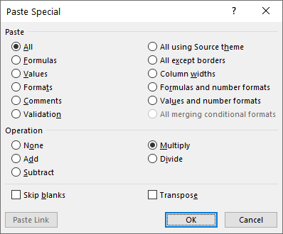
• Click Paste > Paste Special …
• In the Paste Special dialog, select Operation > Multiply
• Click OK

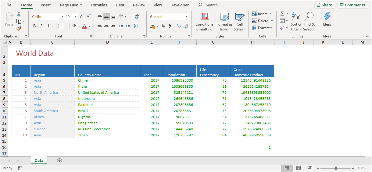
After you click OK, the selected text numbers are multiplied by one, keep their original value, but with the formats from the cell that you copied. Apart from the fact that you have to apply the correct border options because the copied cell did not have any borders at all, this is exactly what you want!

Another issue that might occur when you add data, is about phantom spaces. Consider an imaginary fixed-width text file with some data about countries in the world. This file contains the Region field. The length of this field is 15 characters. I can import this file into Excel and use it as the default list for my analysis. The first three records in Figure 3‑5 are records from this imported fixed-width text file. Although you don’t see it, the region name of these three records contains 15 characters. So, when you read North America, the actual value is North America, with 2 added spaces.

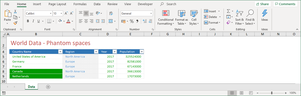
I can add additional data to update my table, which is exactly what I have done. In Figure 3‑5, I have added data to the table. As there is no reason to add country names or regions with extra spaces, I added Canada for North America and Netherlands for Europe. Just the country name and the region. No extra spaces!

When I use an autofilter to select a region, I don’t see anything strange. I expect two regions, and I find two regions.

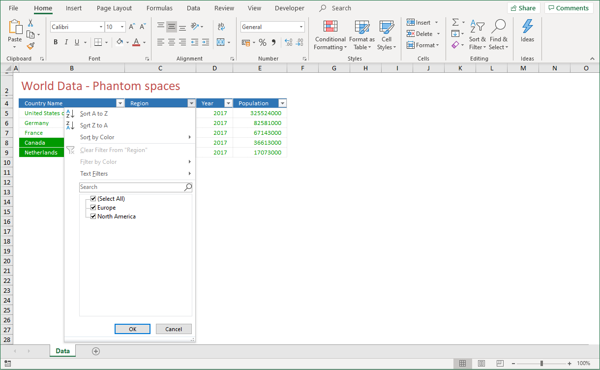
You might wonder why I get into this, as this seems quite normal. But is it? In this case, I know that I have two entries for North America. The same goes for Europe. There is one entry with added spaces and one entry without added spaces. These are totally different entries, but strangely, the autofilter treats them equally.

I take it that you are familiar with pivot tables. Besides some powerful statistical features that this tool offers, a pivot table can also be used to do some serious error checking.

Take a look at what happens when I create a pivot table from my report. Instead of two regions, I get four! Based on my previous experience with the autofilter, and because I created the same analysis, I would expect two regions! Now, who is fooling whom?

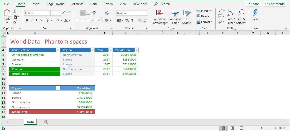
The pivot table analysis can’t be wrong, as I indeed have two entries for North America. The same goes for Europe. There are entries with and without added spaces. That makes four regions. So, in my opinion it is this analysis, and thus the pivot table, that gives the correct answer.

That being said, I don’t know why these two identical analyses give different answers. The Excel team at Microsoft must have had a good reason to implement this, as I can’t think of me being the only one having noticed it.

On the other hand, it might be an advantage to have different answers to the same analysis as I can use this inconsistency for error checking options!

For now, I just need to clear those “excess” spaces. Is there an Excel function to achieve that?

Excess spaces can be removed with the TRIM function. Excess spaces are spaces before and after a “text string”. The TRIM function does NOT remove spaces between words.

The TRIM function was designed to remove the 7-bit ASCII space character (value 32) from text. In the Unicode character set, there is another space character called the non-breaking space character. It has a decimal value of 160. This character is used in Web pages as the HTML entity,  . The TRIM function does NOT remove this non-breaking space character.

You can find the TRIM function in the TEXT category in the function library. From the Formulas Tab, select Function library > Text > TRIM.

SYNTAX

=TRIM(Text)

The TRIM function has one argument:

• Text        The text (in a cell) from which you want to delete the excess spaces

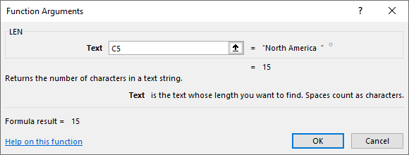
Figure 3‑8 shows the result of the TRIM function. The excess spaces to the right of the string “North America ” are removed.

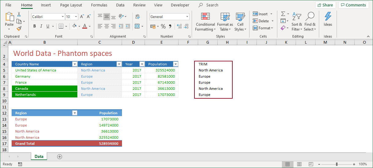
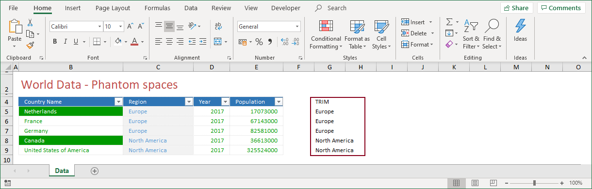
So, now you know how it works, let’s insert the TRIM function into the report shown in Figure 3‑5. The best way is to put it to the right of the table, next to population.

• Select the cell next to population
• Type =TRIM(
• Select the cell with the text you want to remove the excess spaces from
• Type ), and press Enter
• Double-click the fill handle (the dot at the bottom right of the selected cell) to automatically copy the function to the other cells

After completing these steps, the report looks as follows:

The last thing to do is replace the old list of regions with the new or trimmed list of regions.

• Select the new “trimmed” entries
• Click Copy
• Select the first entry in the Region column
• Click Paste > as Values
• Click OK

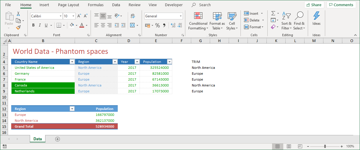
The result is a list of regions that is replaced with trimmed entries. The good thing about this, is that you won’t see it. The bad thing about this, is also that you don’t see it. So, how do I know if it worked?

The pivot table will give the answer!

• Right-click a cell from the pivot table and click Refresh

The pivot table updates the changes and will show only two regions, which is what you expect.

The Trim function is a handy feature to remove excess spaces, but how do you know if there are excess spaces to remove anyway? Actually, you don’t, but in case you get your data from an external source, it is one of those things that you should check before you start analyzing the data. Excel has a function that can give you an indication about possible excess spaces. That function is called LEN.

You can use the LEN function to determine the length of a text string. This is particularly handy in Figure 3‑5, where you can use this function on the Region field to determine the length of the region names and thus see the difference.

You can find the LEN function in the Text category in the function library. From the Formulas tab, select Function library > Text > LEN.

SYNTAX

=LEN(Text)

The LEN function has one argument:

• Text        The text (in a cell) from which you want to delete the excess spaces

The best way to use the LEN function is on a sorted table. This makes it easy to compare non identical entries.

In Figure 3‑12, the data is sorted by Region and Country Name. The experienced user would immediately see that this sort is not correct, for if it was, the entry Netherlands would not have been listed before France and Germany, but after. This could only mean that the three entries for Europe are not identical (as we know).

To find the difference between these entries, use the LEN function on the Region field.

• Select the cell next to population
• Type =LEN(
• Select the cell with the text you want to know the length of
• Type ), and press Enter
• Double-click the fill handle (the dot at the bottom right of a selected cell) to automatically copy the function to all of the other cells

After this operation, the table looks like this:

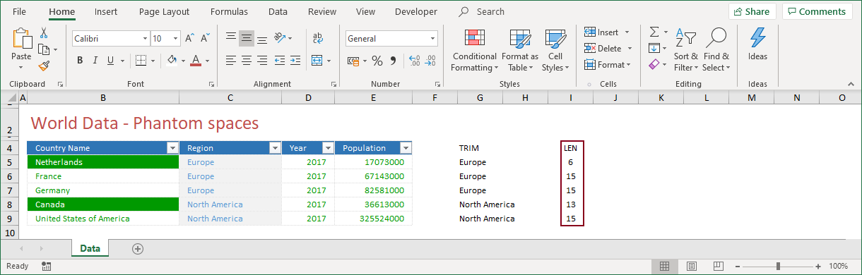
Figure 3‑13 shows why the sort didn’t work out as expected. The LEN function specifies that both regions are different in length and are thus different entries.

When you have to work with data in Excel, it is essential that you work with valid data. In this article, I stated that when it comes to data and Excel, the best way to behave is to never trust your data. I presented a couple of examples to show how non valid data may become the data that you are about to analyze.

Excel has a couple of ways to check for valid data. I suggest that you at least use one of them when you have to analyze or otherwise work with data.

In case your data is not completely valid, Excel has a couple of tools and functions to convert “invalid” data. Use them, as it will make your daily Excel job less frustrating!

——————

This article is an extract from my book From Data 2 Dashboard in a Day. This book covers many more tools, tips and tricks about data that you use for dashboard reporting with Excel. You can purchase your copy here or see a preview in the book shop.